Tutorial
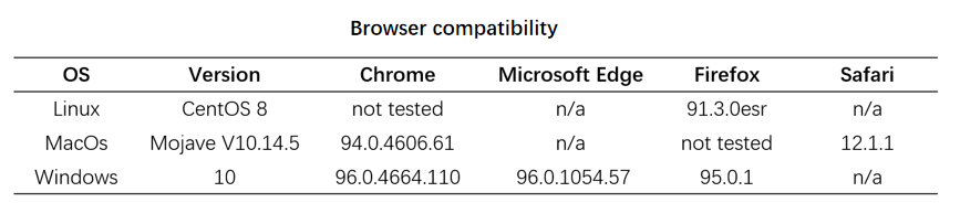
Browser compatibility
File Format
The PED, MAP, phenotype, and sample information files should be named with the suffix of “.ped”, “.map”, ”.phe”, and “.txt”, respectively.
example.ped file:
The ped file is white-space (space or tab) delimited and contains genotypes for each sample. The
first six columns are mandatory: Family ID; Individual ID; Paternal ID; Maternal ID; Sex
(1=male, 2=female, other=unknown); and Phenotype (-9 for missing value). The IDs should only
consist of numbers and letters. Please refer to the format reference for details
(https://www.cog-genomics.org/plink/1.9/formats#ped).

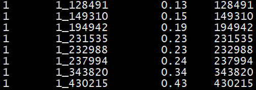
example.map file:
The map file is white-space delimited and includes four columns: chromosome ID, SNP ID, genetic
distance (cM), and genomic coordinates (bp). We recommend users to name the chromosomes with
numbers. Otherwise, the chromosome IDs will be replaced to numbers automatically. The modified
IDs will be stored in the file of “Chr.rename.txt”. Please refer to the format reference for
details (https://www.cog-genomics.org/plink/1.9/formats#map).
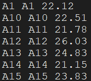
example.phe file:
The phe file is white-space delimited file and includes three columns: family ID, individual ID,
and phenotypes. The phenotype can be continuous or discrete (0 and 1). Please note that only the
phenotype from the 3rd column is extracted for analysis. Please refer to the format reference
for details (https://www.cog-genomics.org/plink/1.9/input#pheno).
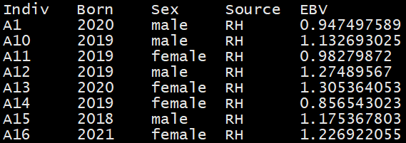
sample_information.txt:
The file has columns of sample IDs , years of birth, genders , source of samples, estimated
breeding values. The headers of every columns must be named as “Indiv”, “Born”, “Sex”, “Source”,
and “EBV”, respectively.
Phenotype Segmentation
Enter the "Smart Breeding" interface from the table tab above.
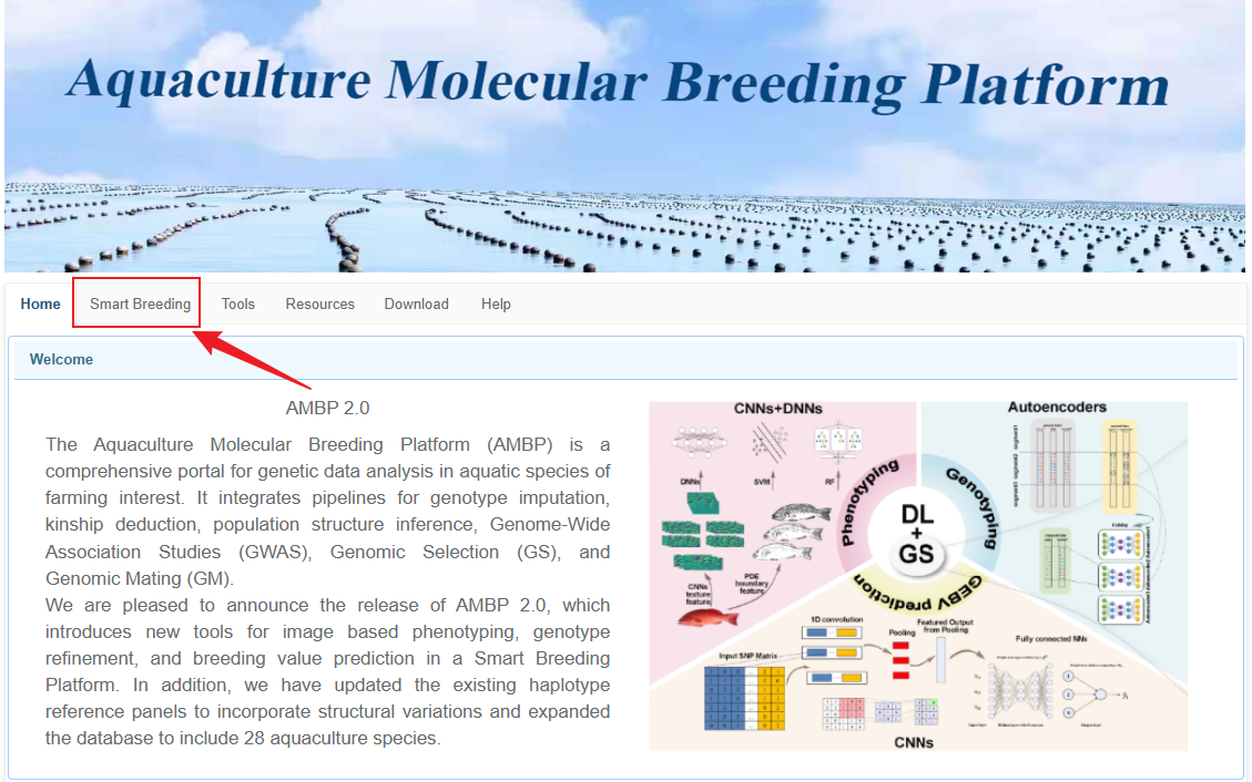
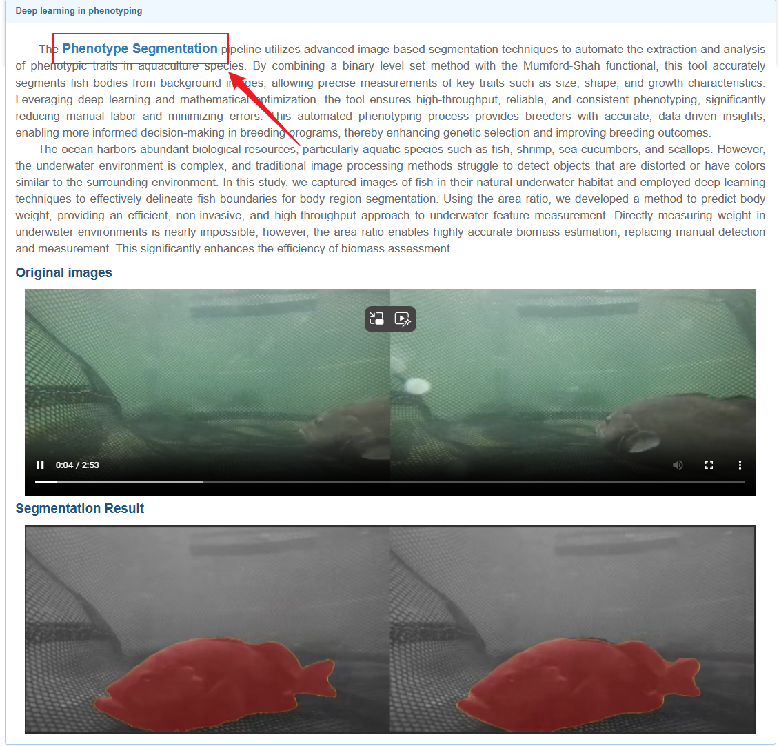
Click on 'Phenotype Segmentation' in the 'Deep Learning in Phenotyping' module to try our underwater phenotype recognition deep learning model. Our model can segment underwater biological photos and roughly measure their phenotype data.
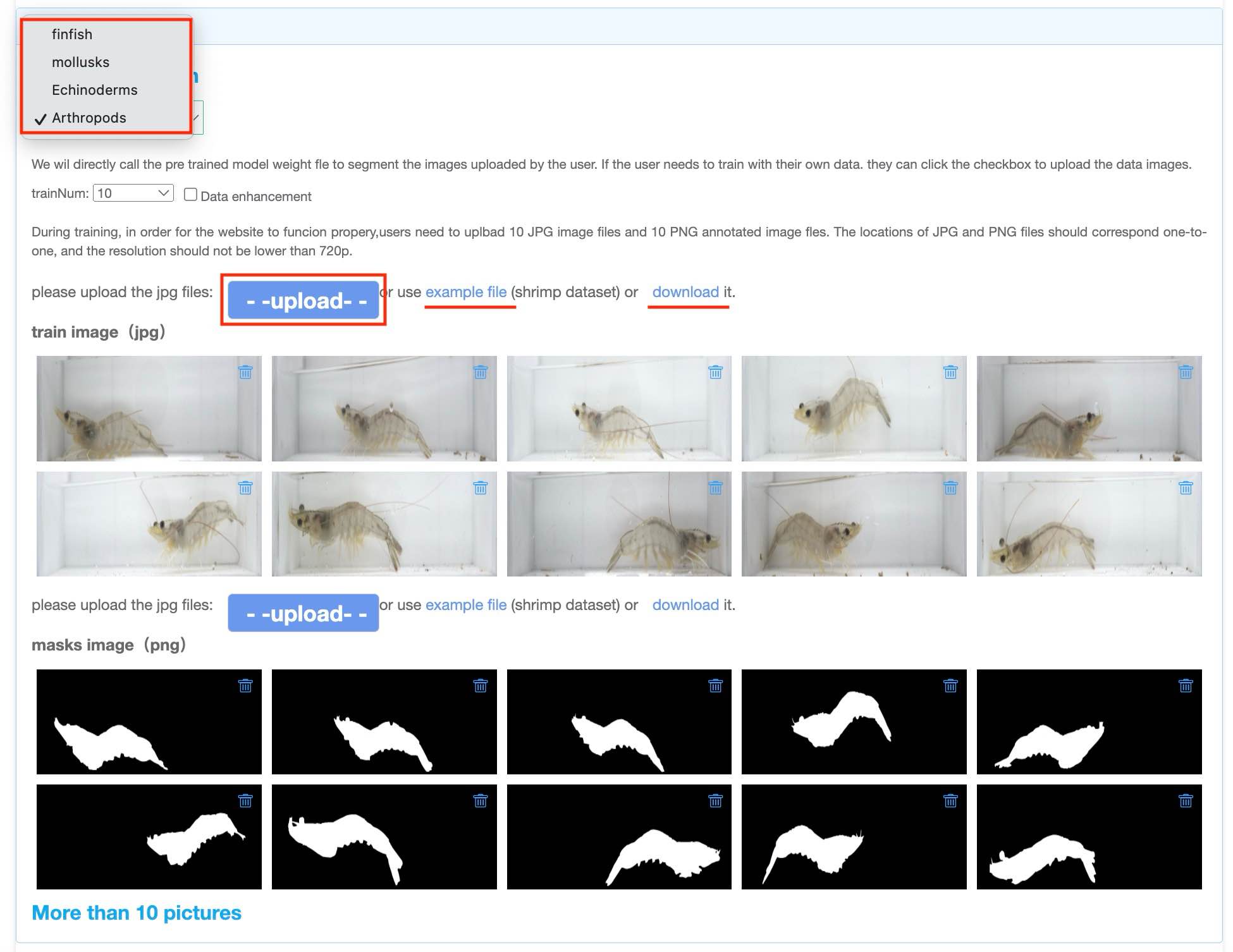
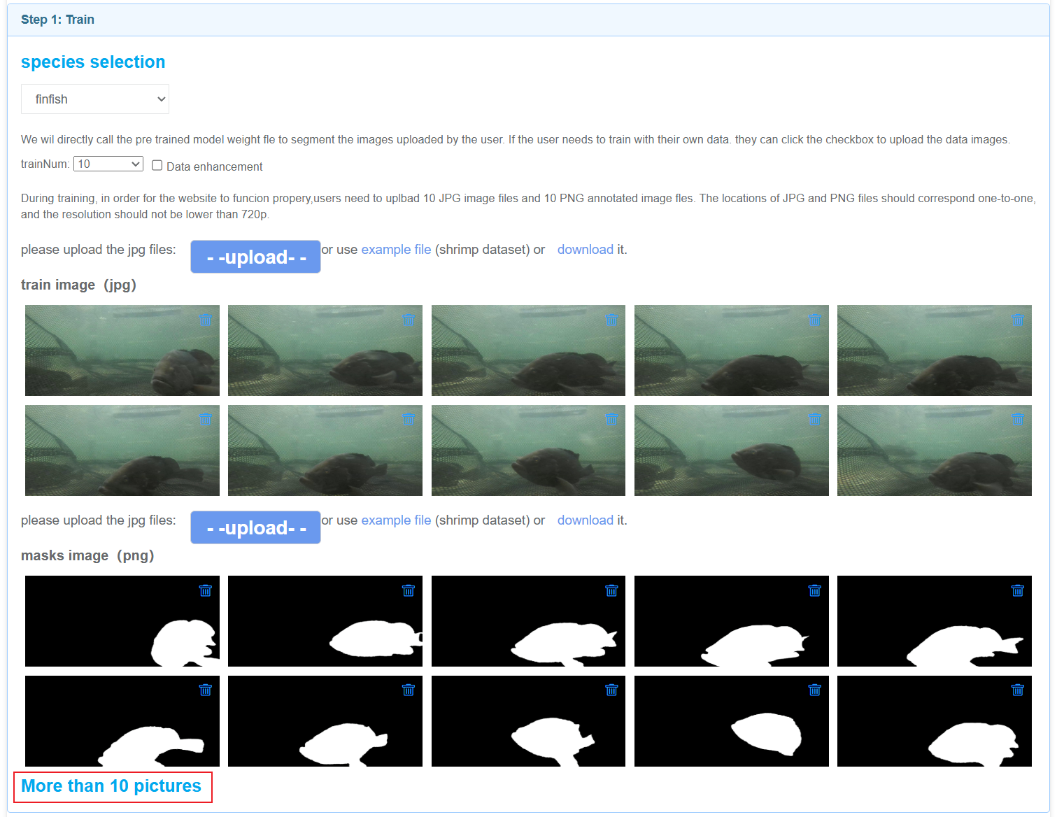
In the first step: train, there are four species to choose from, each corresponding to a set of example images. Users can click "upload" to upload their training data, or click "example file" to use the example data we provide. You can also click "download" to download sample data.
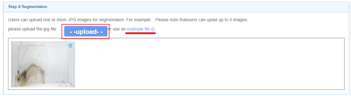
In the second step: Segmentation, users can click "upload" to upload their segmentation data, or click "example file" to use the example data we provide.
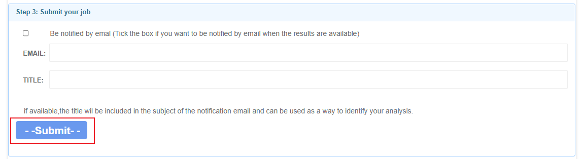
Due to the long training time, users can submit tasks on the website by filling in their email and title. Once the task is completed, the results will be automatically sent to the email address provided by the user.
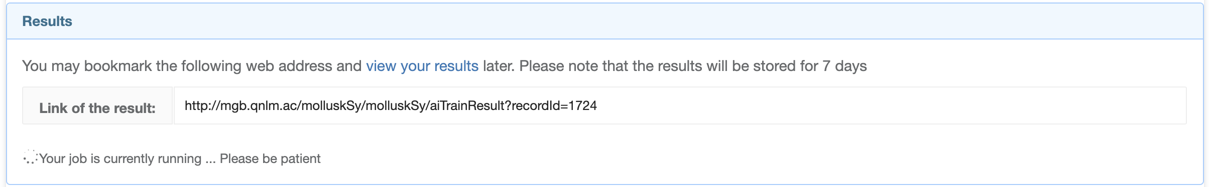
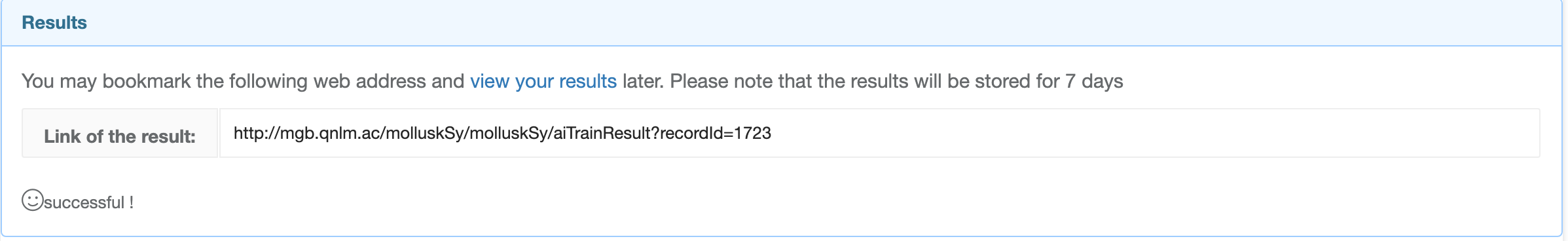
After the task is completed, a link will be generated. Copy the link to the browser and open it to view the running results.
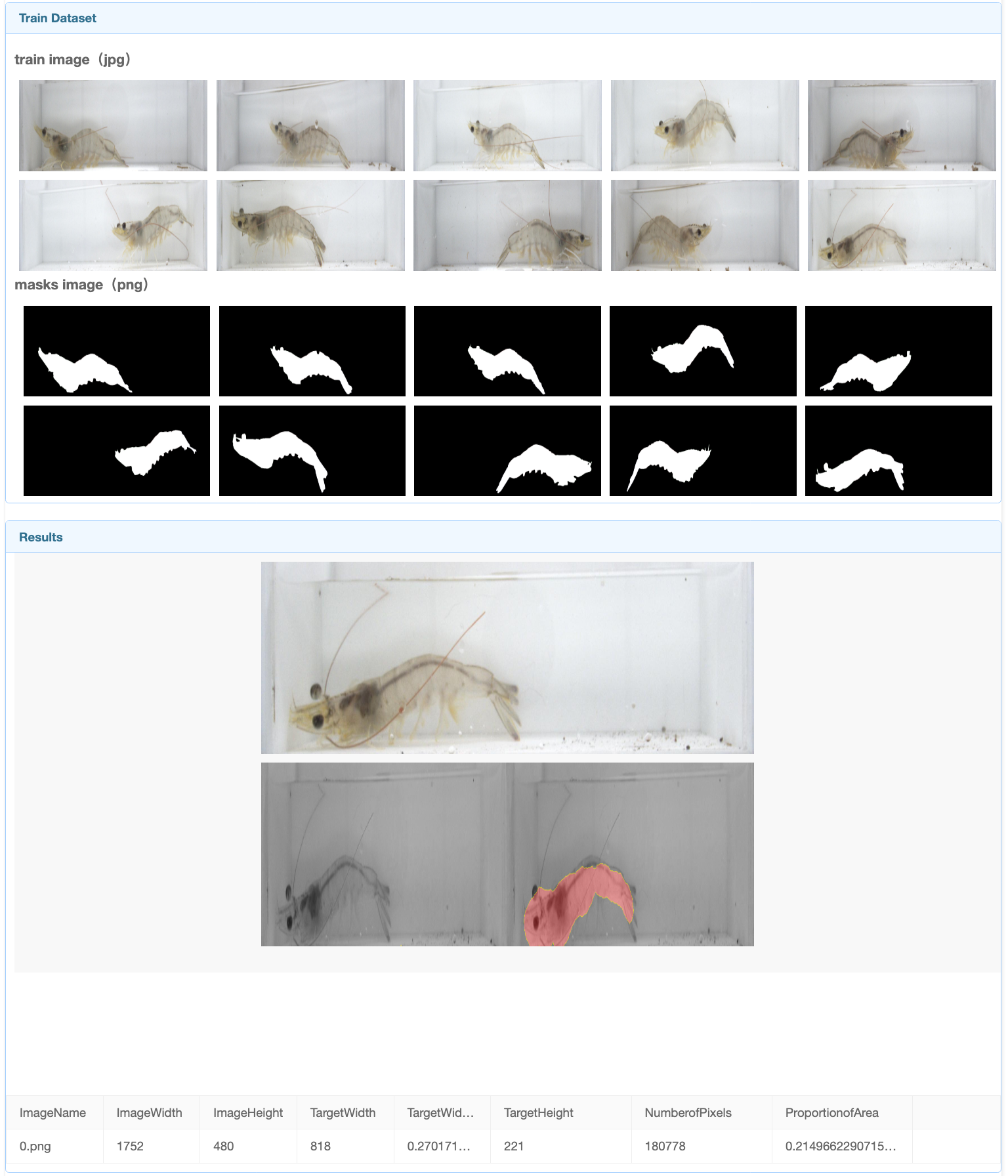
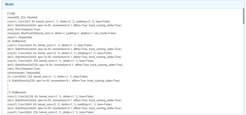
In the final result interface, you can see the images used for training, masks, The segmentation results and partial analysis of the final image can be found at the end of the page, along with information about the model we used.
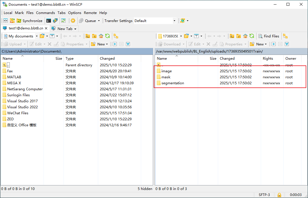
If users need to upload a large amount of data, they can click the "More than 10 pictures" button.
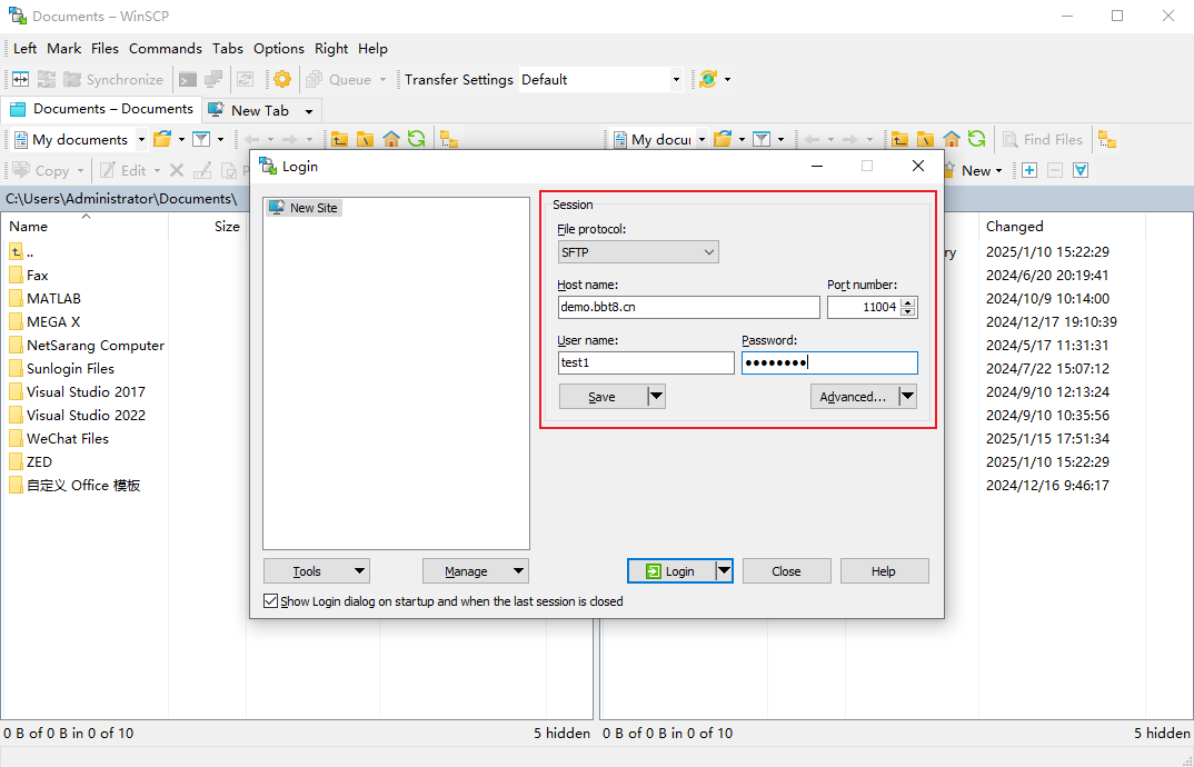
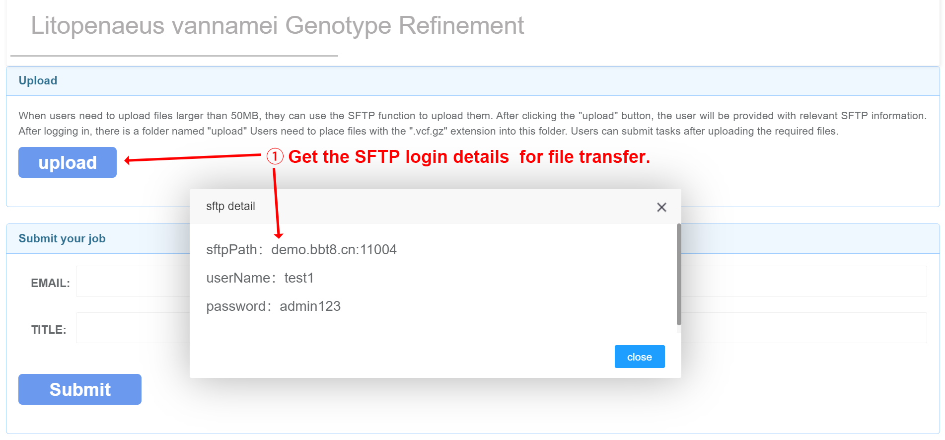
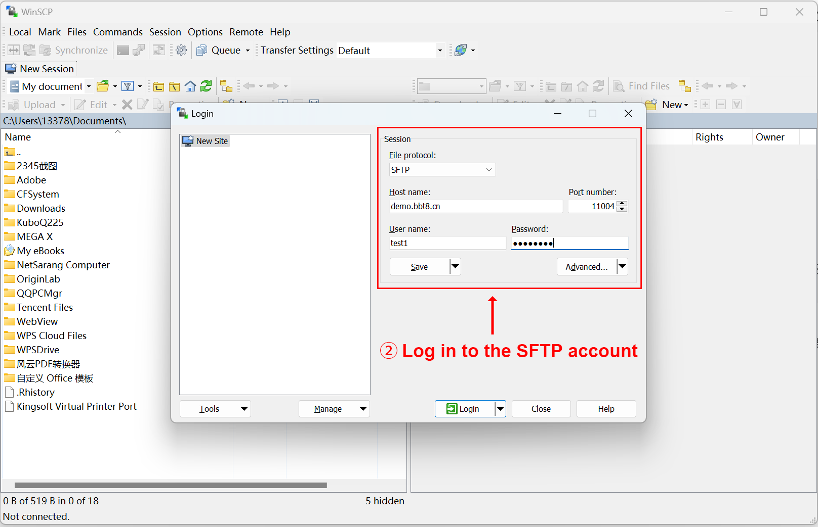
After clicking 'Upload', SFTP related information will be provided, and you can upload files after logging in. We recommend using the software WinSCP. After successful login, upload the corresponding data in the image, mask, and segmentation folders. Users fill in their email and project related information, and after data processing is completed, the results will be sent to the user's email.
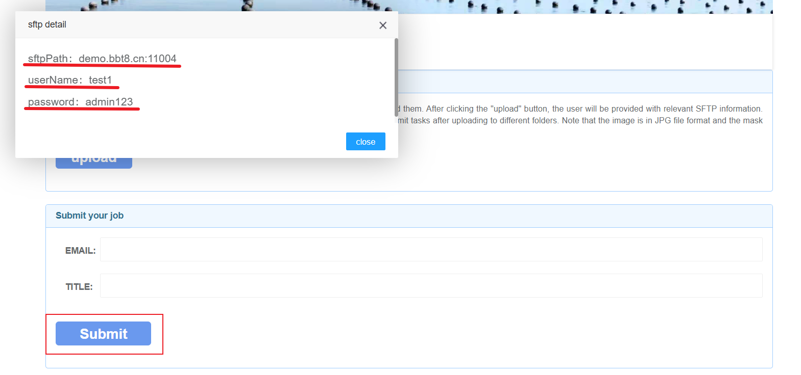
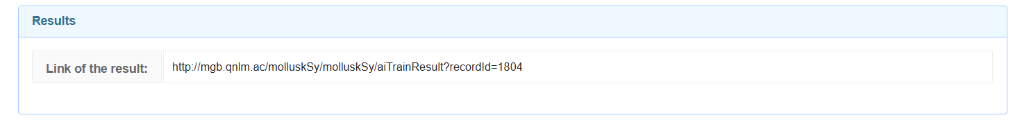
After submitting the task, the user will receive a link, save this link, and after the data processing is completed, they can view the results through this link.
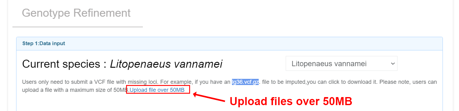
Genotype Refinement
Input files Users can upload VCF files with missing loci and perform online imputation and correction of missing genotype data using a denoising autoencoder model. Note: (1) Your input files should be named as ${chr_name}.vcf.gz. You can check the list of chromosomes for each species on theGenotype Refinement page. Example: lg3.vcf.gz lg36.vcf.gz (2) The header of VCF files should have the information of chromosomes. Example: lg3.vcf.gz lg36.vcf.gz ##contig=<ID=lg3,length=57207694> ##contig=<ID=lg36,length=23119636> (3) The sample IDs should only consist of numbers and letters.
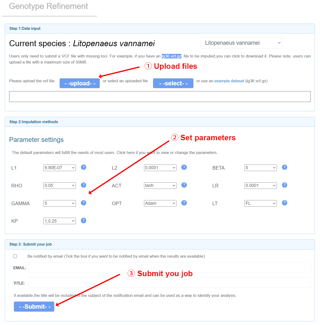
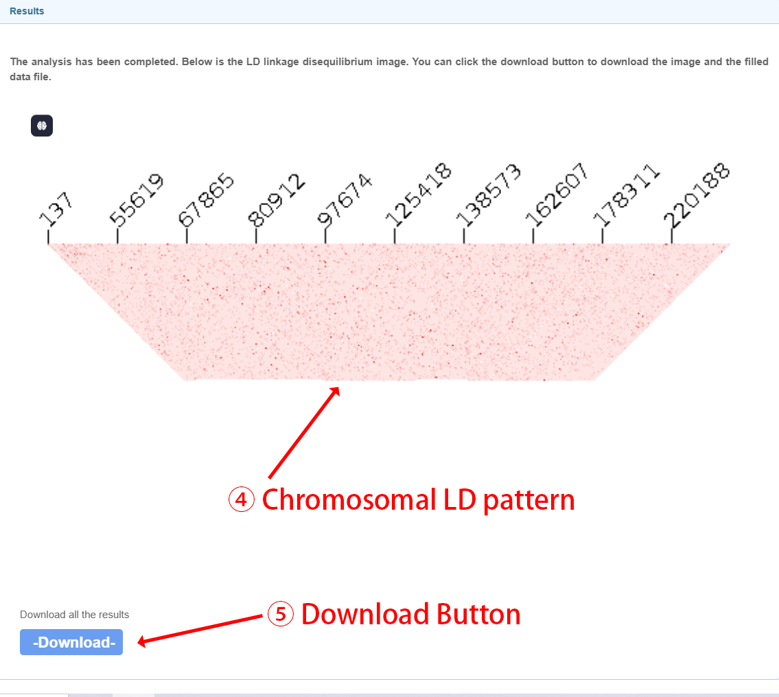
Output files Users will get imputed genotypes in vcf.gz format. A ped file and map file will also be generated for subsequent analysis. The global imputation rate and linkage disequilibrium (LD) patterns will be visually illustrated for chromosomes longer than 2M bp.

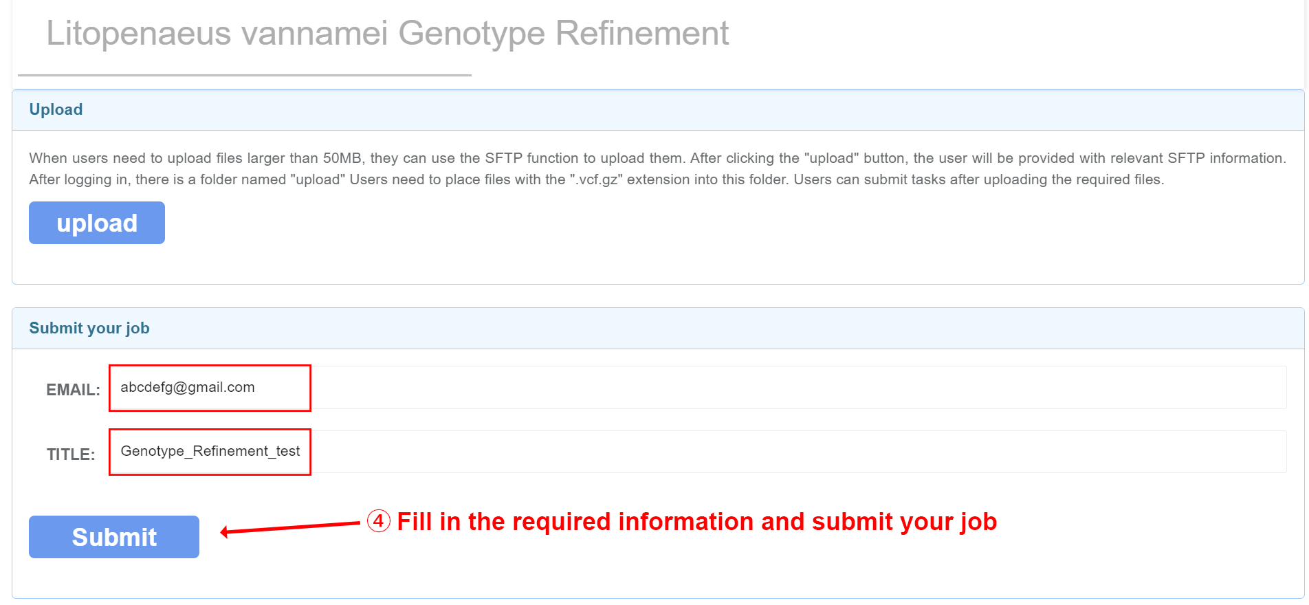
After filling in the required information and submitting your job, the user will receive an email with the attached genotype refinement results file within three days.
GEBV Prediction
Input files GEBV Prediction requires three input files (ped, map, and phe). Please note that the sample ID should only consist of numbers and letters, and the prefixes of the three files should remain consistent. Then, the breeding values can be calculated using three types of neural networks: DNN, CNN, and RNN.

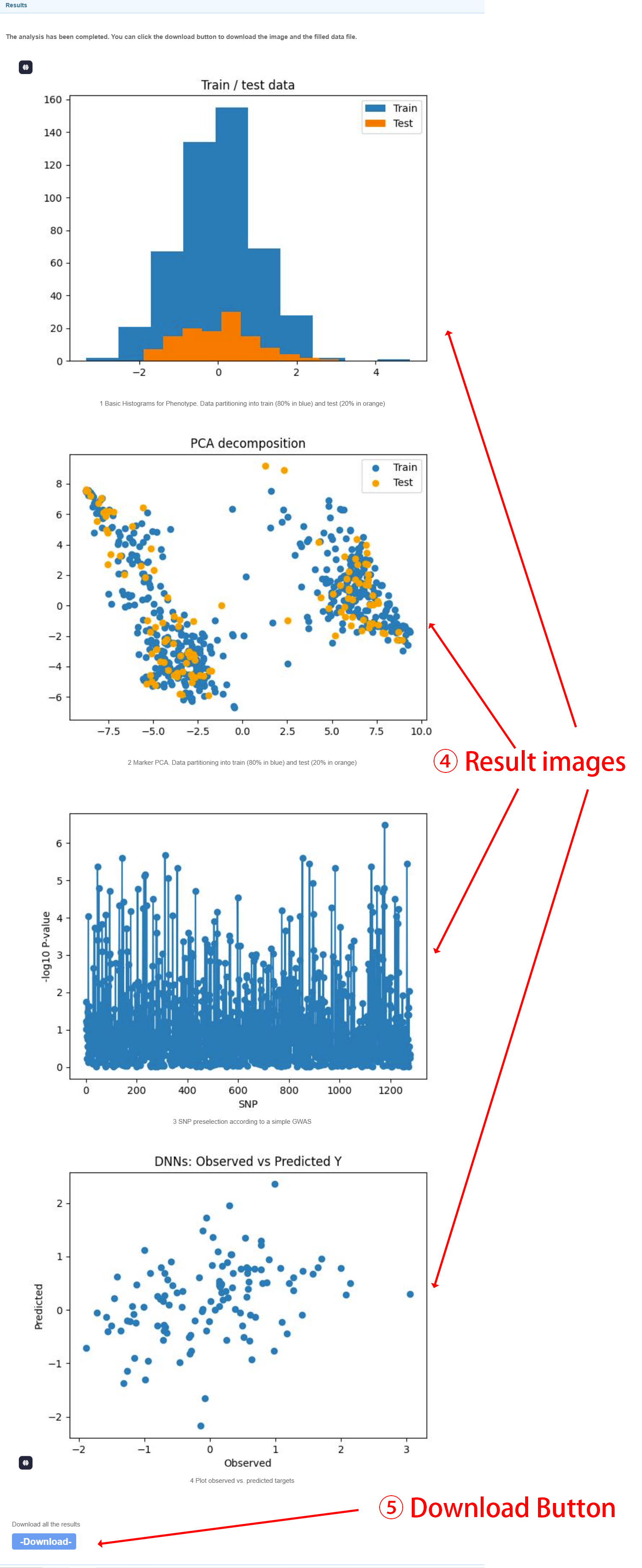
Output files After calculating the breeding values using neural networks, four images will be generated, which are: Basic Histograms for Phenotype、Marker PCA、SNP preselection according to a simple GWAS and Plot observed vs. predicted targets. You can click the download button to download the result file.
Online SNP Imputation
Input files Users can upload one or more VCF files and carry out online imputation with corresponding reference panels by Beagle and Glimpse (Browning, et al., 2018; Rubinacci, et al., 2021). As Glimpse requires the genotype likelihoods (GL) or the phred-scaled genotype likelihoods (PL), please make sure your VCF files contain these fields if you would like to use Glimpse for imputation. And a qualified VCF could be generated by common VCF processing tools such as GATK, ATLAS and bcftools (Li, 2011). For more details, please refer to the manuals of Beagle and Glimpse. Note: (1) Your input files should be named as ${chr_name}.vcf.gz. You can check the list of chromosomes for each species on the Online SNP imputation page. Example: lg3.vcf.gz lg36.vcf.gz (2) The header of VCF files should have the information of chromosomes. Example: lg3.vcf.gz lg36.vcf.gz ##contig=<ID=lg3,length=57207694> ##contig=<ID=lg36,length=23119636> (3) The sample IDs should only consist of numbers and letters.
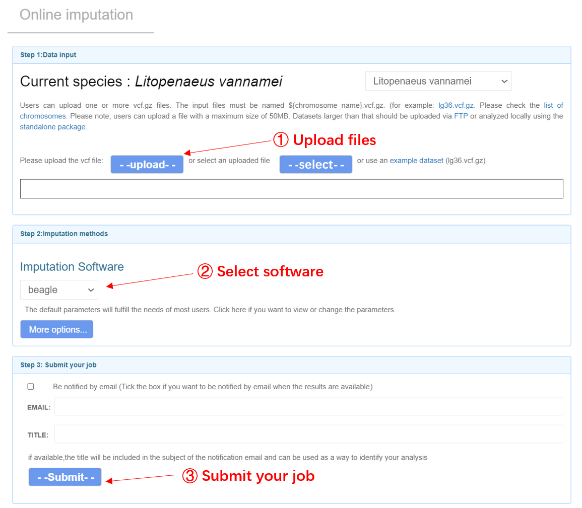
Online imputation web page
Output files Users will get imputed genotypes in vcf.gz format. A ped file and map file will also be generated for subsequent analysis. By default, genotypes with low genotype probabilities (GP) will be filtered. The global imputation rate and linkage disequilibrium (LD) patterns will be visually illustrated for chromosomes longer than 2M bp.

Online imputation results
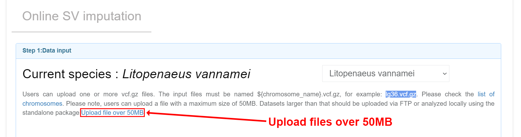
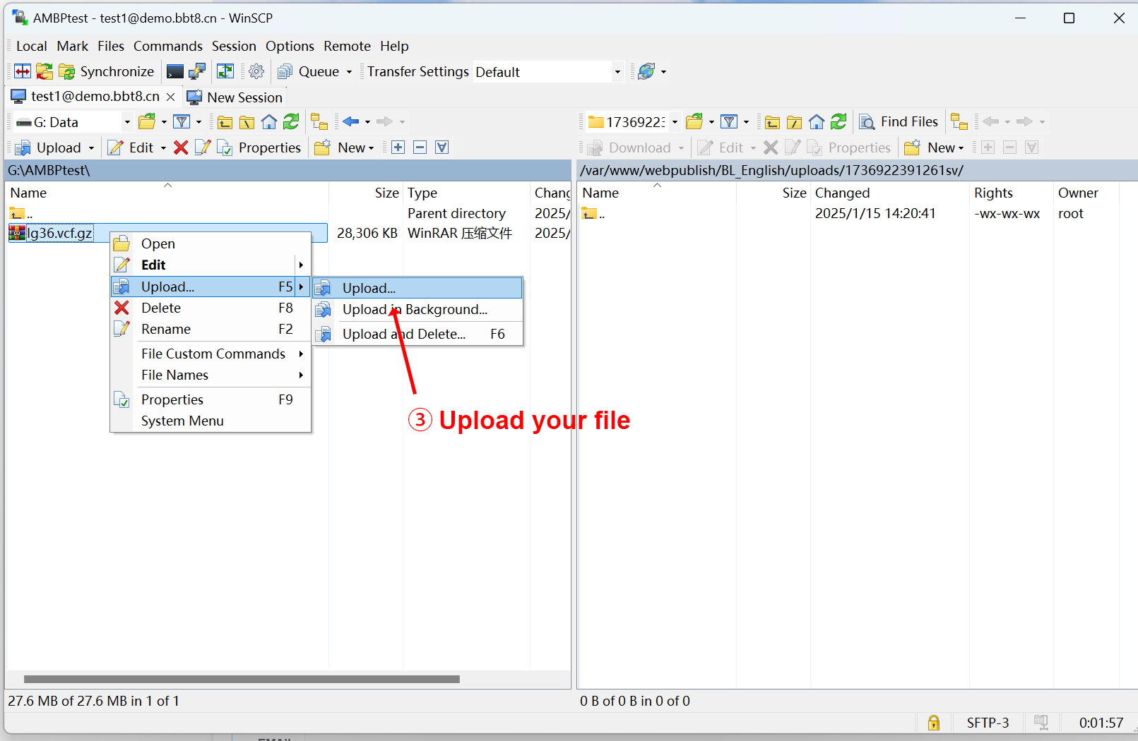
Online SV Imputation
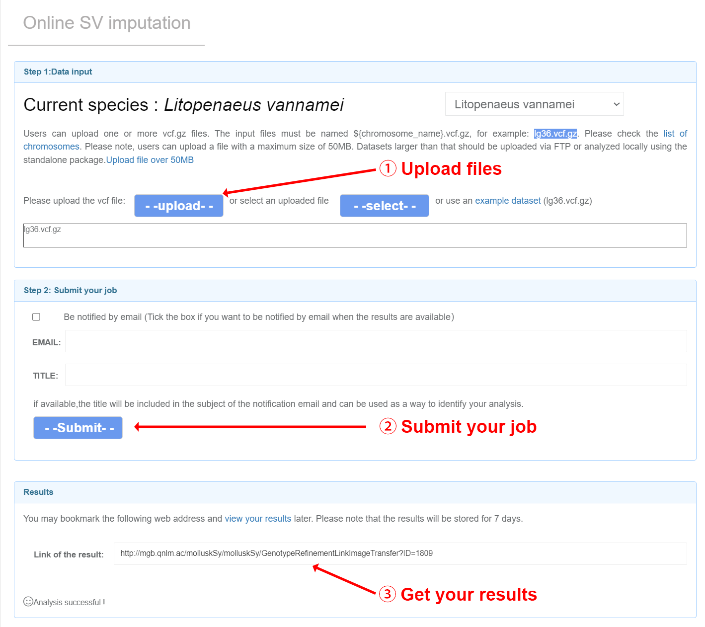
Input files Users can upload one or more VCF files and carry out online imputation with corresponding reference panels by Beagle (Browning, et al., 2018). And a qualified VCF could be generated by common VCF processing tools such as GATK, ATLAS and bcftools (Li, 2011). For more details, please refer to the manuals of Beagle. Note: (1) Your input files should be named as ${chr_name}.vcf.gz. You can check the list of chromosomes for each species on the Online SV imputation page. Example: lg3.vcf.gz lg36.vcf.gz (2) The header of VCF files should have the information of chromosomes. Example: lg3.vcf.gz lg36.vcf.gz ##contig=<ID=lg3,length=57207694> ##contig=<ID=lg36,length=23119636> (3) The sample IDs should only consist of numbers and letters.
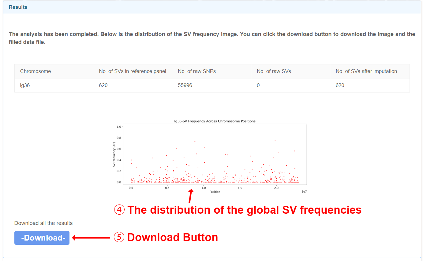
Users will get imputed genotypes in vcf.gz format. A ped file and map file will also be generated for subsequent analysis. The distribution of the global structural variant (SV) frequencies will be visually illustrated for all chromosomes exceeding 2 million base pairs in length.


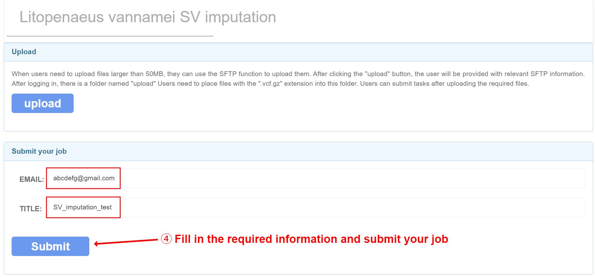
After filling in the required information and submitting your job, the user will receive an email with the attached SV imputation results file within three days.
Genetic Structure Inference
Input file Genetic structure inference requires three input files: genotypes (ped), marker positions (map), and sample_information (txt, optional). Please refer to the File Format section for details. The sample_information should contain columns of “Indiv” and “Source”. The sample IDs should only consist of numbers and letters.

Genetic Structure Inference web page
Output results
Ancestry estimation and principal component analysis will be performed to infer the
population
structure (Alexander, et al., 2009; Purcell, et al., 2007). The optimal number of
ancestries
will be checked by cross-validation.
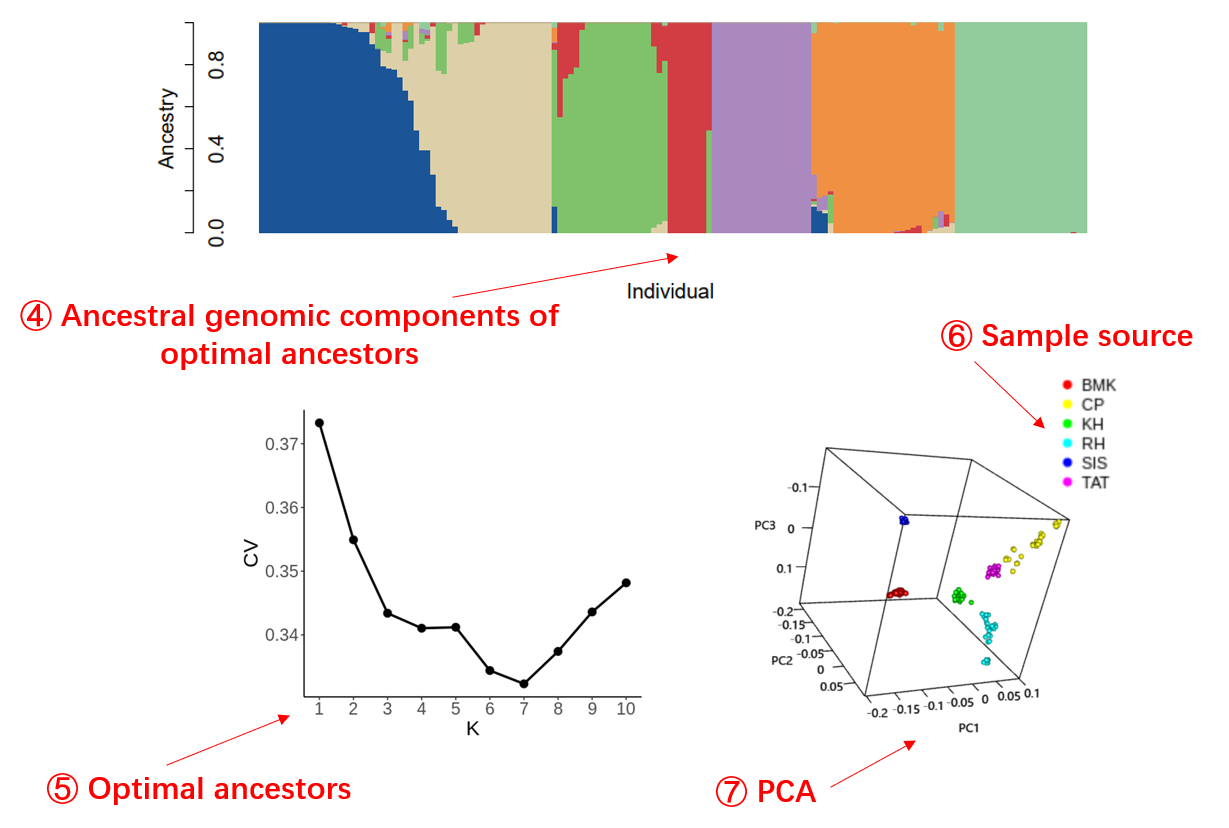
Genetic structure inference results
Kinship
Input filesKinship analysis requires two input files (ped, map) to identify pairwise identical by descent (IBD) segments and estimate pairwise kinship coefficients.
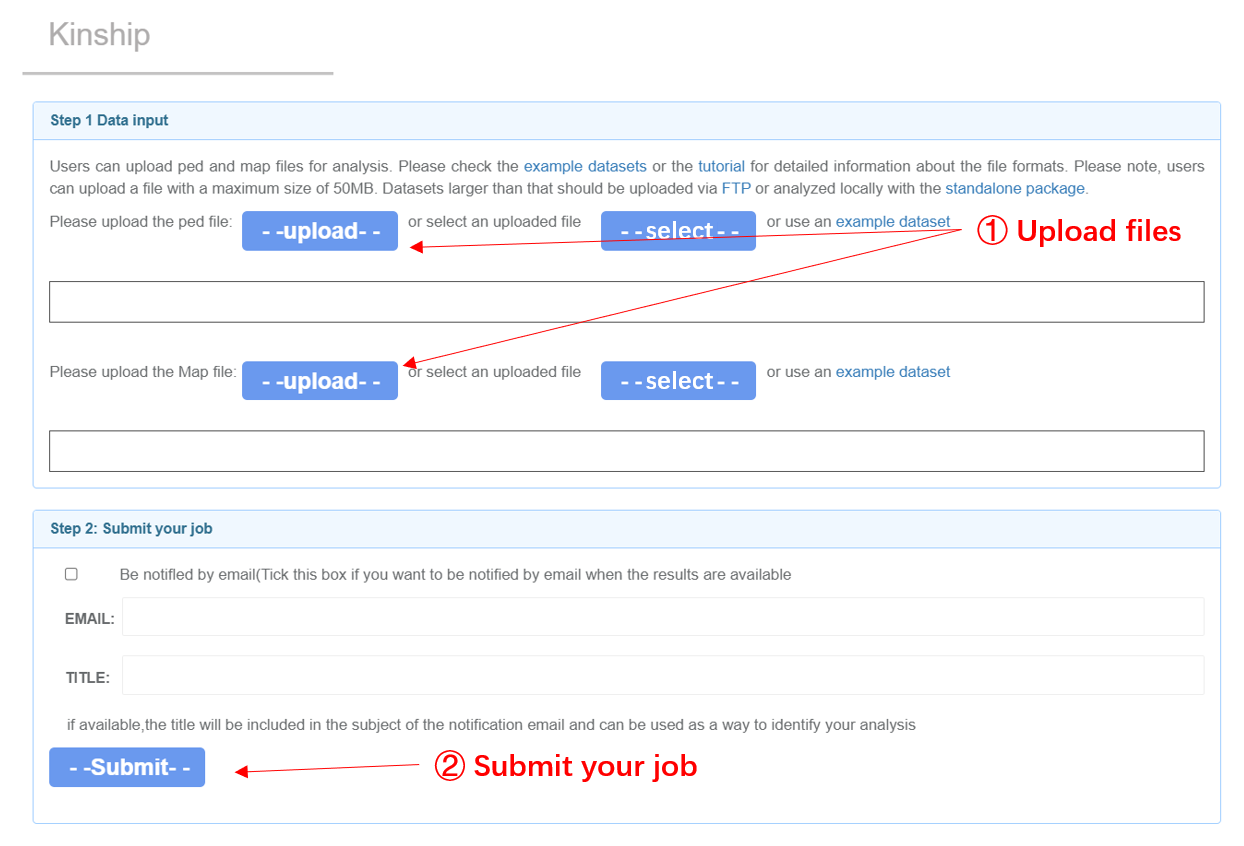
Kinship analysis page
Output files Relationships between the individuals of the population will be evaluated by KING (Manichaikul, et al., 2010). The kinship coefficient of each pairs will be plotted against the proportion of SNPs with two different alleles (IBS0). All pairs will be classified into five degrees: duplicate/monozygotic twin, full sib/parent–offspring, 2nd-degree (such as half-sibs), 3rd-degree (such as first cousins), and unrelated relationships. The results could also be downloaded in tabular format.
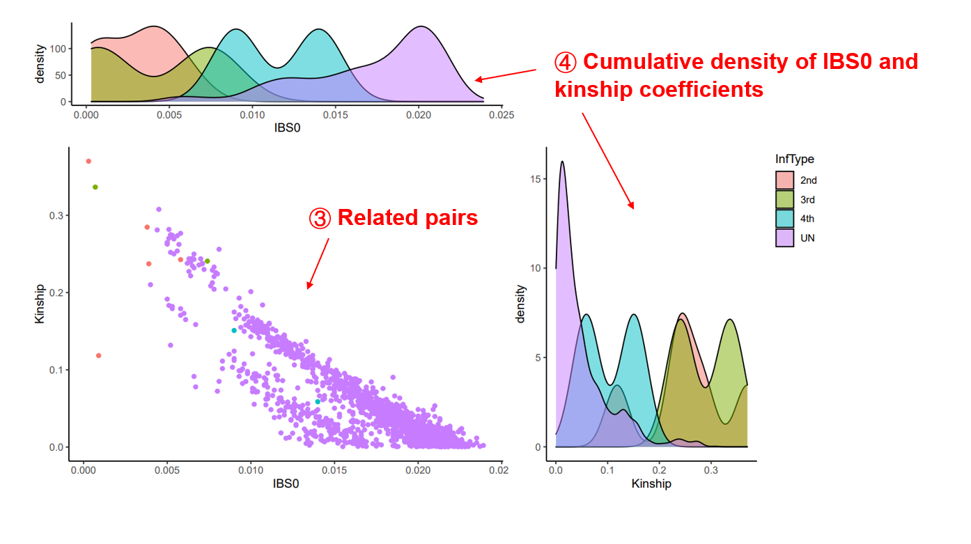
Kinship analysis results
GWAS
Input files GWAS requires three input files (ped, map, and phe). Please note that the sample IDs should only consist of numbers and letters. Pairwise linkage disequilibrium (LD) of SNPs were measured as the squared correlation between phased alleles (r2). By default, r2 threshold of 0.5 was applied to prune SNPs in relatively high LD. Loci with missing rate over 20% will also be trimmed. Genome-wide association analysis will be conducted using a univariate linear mixed model with centered relatedness matrix (Zhou, Stephens, 2012).
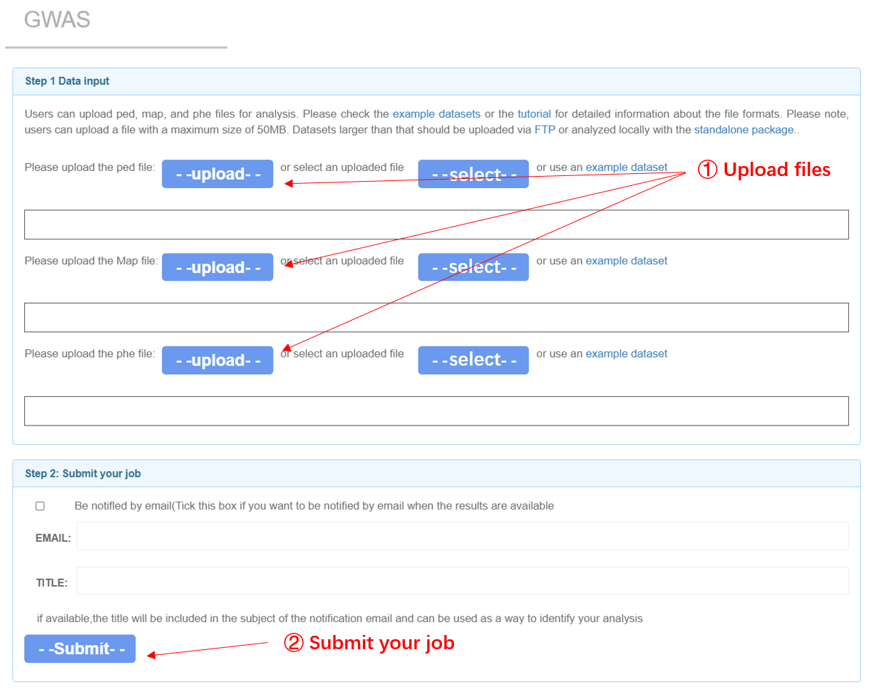
GWAS analysis page
Output results Statistical significance of association will be evaluated by Wald test and illustrated in a Manhattan plot. The pipeline will also exhibit the deviations of the observed P values from the expectations of a theoretical uniform distribution in a QQ plot. The result could be downloaded in tabular format, which contains 11 columns: chromosome numbers, SNP ID, base pair positions on the chromosome, number of missing values for a given SNP, minor allele, major allele, allele frequency, beta estimates, standard errors for beta, remle estimates for lambda, and P values from Wald test.

GWAS analysis results
Genomic Selection
Input files GS analysis uses dataset from the reference population and prediction population. The input files for the reference and candidate population should be prepared separately and have an identical set of genetic markers. The PED, MAP, and phenotype files for the reference population should be named as “mydata.ref.ped”, “mydata.ref.map”, and “mydata.ref.phe”. The PED and MAP files for the candidates should be named as “mydata.predict.ped” and “mydata.predict.map”. Please note that the sample ID should only consist of numbers and letters. We implanted three models (GBLUP, GBayes, SNN) to predict the genomic estimated breeding values (GEBV) (Wang, et al., 2018; Wimmer, et al., 2012). By default, r2 threshold of 0.5 was applied to prune SNPs in relatively high LD. Loci with missing rate over 20% will also be trimmed.User can also enable10-fold Cross-validation on reference dataset in step 3.
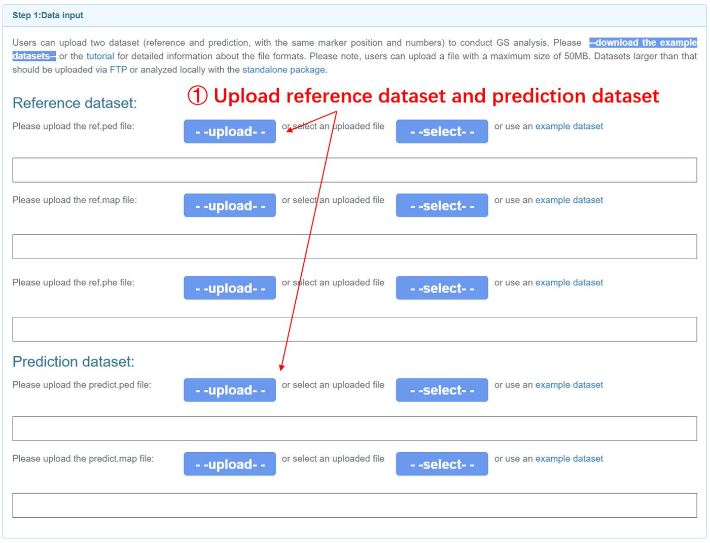

Genomic Selection analysis page
Output files
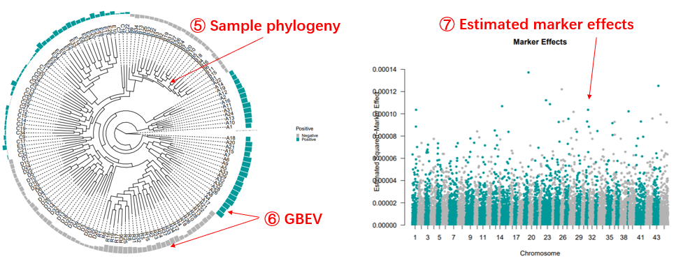
The predicted GEBVs will be illustrated according to the sample phylogeny. The estimated
marker
effects will also be shown to facility inspecting markers of interest. The result could
be
downloaded in tabular format. Users can retrieve the GEBV from the results for
subsequent GM
analysis.
Genomic Selection analysis page
Genomic Mating
Input files GM analysis requires four input files: genotypes (ped), marker positions (map), phenotype (phe), and sample_information (txt). Please refer to the File Format section for details. The file of sample_information should contain columns of “Indiv”, “Born”, and “Sex”. The sample IDs should only consist of numbers and letters. Users can include the pre-calculated GEBVs in the column named “EBV”. Otherwise, the pipeline will calculate GEBV with GBLUP. By default, r2 threshold of 0.5 was applied to prune SNPs in relatively high LD. Loci with missing rate over 20% will also be trimmed.
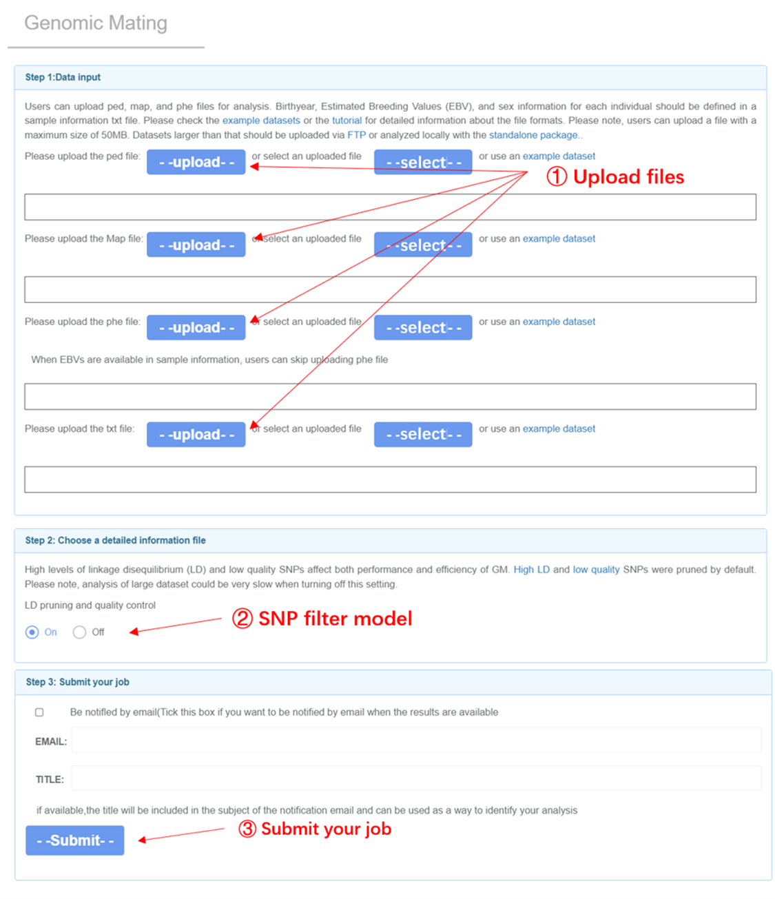
Genomic Mating analysis page
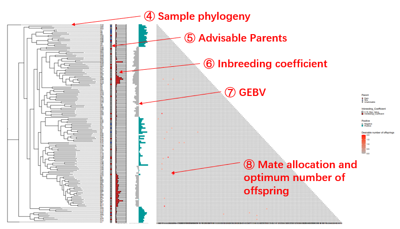
Output results The optimum contribution selection (OCS) and mating strategy will be made according to maximum genetic gain with a constraining increase in mean kinship (Wellmann, 2019). The threshold for a kinship K is set according to the formula:
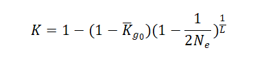
Where Kg0 is the mean kinship in the population at generation g0, L is the generation interval in years. By default,Ne is set as 200 to avoid inbreeding depression. The mate allocation and optimum number of offspring will be illustrated in a heatmap and a chord plot. The results could also be downloaded in tabular format.
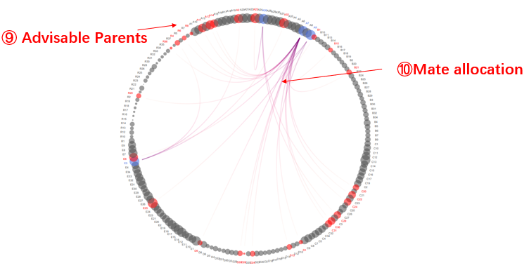
Genomic Mating analysis results
Simulation
Input files Simulation analysis requires four input files: genotypes (ped), marker positions (map), phenotype (phe). Please refer to the File Format section for details.

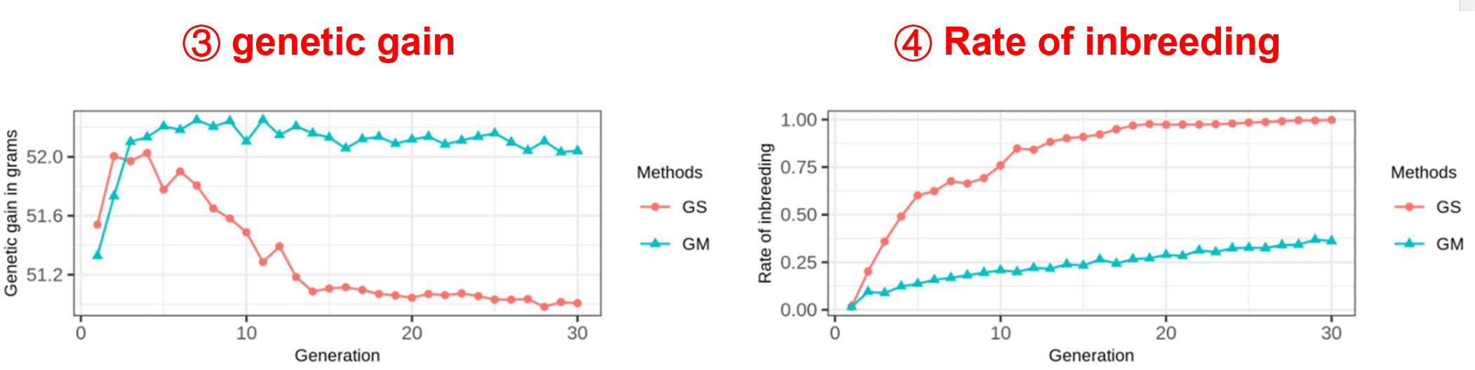
Output results The simulation results of 30 generations will be output. And the genetic gain and rate of inbreeding will be displayed.
Local Installation
1.Acquire Docker image from Docker hub.
docker pull ouc2021mgb/ambp:latest2.For genotype imputation, please download the reference panel of interest from the server and move them to the directory that will be mounted in the docker container.
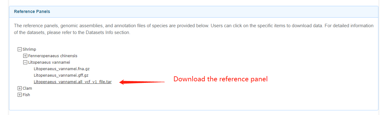
Download the reference panel
mkdir -p /host_path/host_analysis/reference_panel/L_vannamei
mv Litopenaeus_vannamei.all_vcf_v1_file.tar /host_path/host_analysis/reference_panel/L_vannamei
tar -xvzf /host_path/host_analysis/reference_panel/L_vannamei/Litopenaeus_vannamei.all.vcf.tar
3. Prepare your input files according to the tutorial above and move them to the directory that will be mounted in the docker container.
mkdir -p /host_path/host_analysis/impute_example
mv input.vcf.gz /host_path/host_analysis/impute_example

Prepare the input data for imputation
4. Prepare a config file, you can download the template file and adjust it to fit your analysis. The config file should be deposited in the directory that will be mounted in the docker container.
mkdir -p /host_path/to/host_analysis/impute_input
mv allinputfile.vcf.gz /host_path/host_analysis/impute_input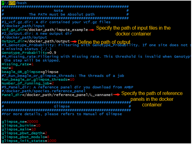
Adjust the config file
5. Analyze your data in the docker container.
docker run -v /host_path/host_analysis/:/docker_path/ -it ouc2021mgb/ambp:latest /bin/bash /docker_path/imputation.config Reference
Alexander, D.H., Novembre, J., Lange, K., 2009. Fast model-based estimation of ancestry in unrelated individuals. Genome Research. 19, 1655-1664. Browning, B.L., Zhou, Y., Browning, S.R., 2018. A One-Penny Imputed Genome from Next-Generation Reference Panels. Am J Hum Genet. 103, 338-348. Li, H., 2011. A statistical framework for SNP calling, mutation discovery, association mapping and population genetical parameter estimation from sequencing data. Bioinformatics. 27, 2987-2993. Manichaikul, A., Mychaleckyj, J.C., Rich, S.S., Daly, K., Sale, M., Chen, W.M., 2010. Robust relationship inference in genome-wide association studies. Bioinformatics. 26, 2867-2873. Purcell, S., Neale, B., Todd-Brown, K., Thomas, L., Ferreira, M.A., Bender, D., Maller, J., Sklar, P., De Bakker, P.I., Daly, M.J., 2007. PLINK: a tool set for whole-genome association and population-based linkage analyses. The American journal of human genetics. 81, 559-575. Rubinacci, S., Ribeiro, D.M., Hofmeister, R.J., Delaneau, O., 2021. Efficient phasing and imputation of low-coverage sequencing data using large reference panels. Nat Genet. 53, 120-126. Wang, Y., Mi, X., Rosa, G.J.M., Chen, Z., Lin, P., Wang, S., Bao, Z., 2018. Technical note: an R package for fitting sparse neural networks with application in animal breeding. J Anim Sci. 96, 2016-2026. Wellmann, R., 2019. Optimum contribution selection for animal breeding and conservation: the R package optiSel. BMC Bioinformatics. 20, 25. Wimmer, V., Albrecht, T., Auinger, H.J., Schon, C.C., 2012. synbreed: a framework for the analysis of genomic prediction data using R. Bioinformatics. 28, 2086-2087. Zhou, X., Stephens, M., 2012. Genome-wide efficient mixed-model analysis for association studies. Nat Genet. 44, 821-824.